Compose interesting VFX by combining shader functions

Mathematical functions lay as the foundation of most shaders. As a shader artist, your job is to use these abstract equations to gain control over shaping the effects you're creating.

While individual functions are incredibly powerful on their own, using them in isolation only gets you so far. The real magic happens when you start blending them together. By adding, multiplying, or nesting functions inside each other, you can construct complex, believable animations.

You can turn simple oscillations into natural looking ocean waves:

Or, you can control the rate at which an oscillation grows to create ripples, or even flatten a repeating pattern's values to create retro stylized rings:

And once you master combining functions, you can mark the occasion with a fluttering flag. Just make sure you pin it to its pole first!

In this guide, you'll learn how to combine shader functions to build more interesting effects!

You will be able to:

• Create visual complexity by making use of simple addition
• Reshape functions with multiplication
• Selectively animate parts of a shader
• Use function composition to change the feel of an effect

Shaping effects with Math

Before we start mixing functions together, let's do a quick recap of how a single function maps onto a shader. If you want a deep dive into individual functions, check out the full guide on how to control shaders with functions.

At its core, a mathematical function defines a relationship between two values. For example, the identity function $y=x$ means that whatever goes in for $x$ comes out exactly the same for $y$.

Inside a shader, these $x$ and $y$ values, or better named, the function input and output, can represent anything. For example, you can use the horizontal coordinate of a pixel (UV.x) in order to generate a grayscale color:

void fragment() {
  float y = UV.x;
  vec3 gradient = vec3(y);

  COLOR = vec4(gradient, 1.0);
}

How do I get the coordinates of a pixel?

Unlike regular code, a shader program doesn't process the whole image. Instead, it runs once for every pixel. To help you tell pixels apart, Godot provides built-in variables such as UV, which describes the current pixel's position.

UV coordinates are a broader topic than this guide covers. If you'd like to learn more, you can read about them in the library. For the purposes of this lesson, simply think of UV as the current pixel's position, with both coordinates ranging from 0.0 to 1.0.

In the shader above, UV.x is the horizontal coordinate. For pixels on the left this value gets closer to 0.0, while for pixels on the right it approaches 1.0. You can use it to create a vector of three elements which maps to the red, green and blue channels of the final color. This produces a smooth grayscale gradient across the sprite. The last component of the COLOR built-in represents the alpha, or transparency. For a fully visible gradient, you can leave that to 1.0.

Visualizing functions inside a shader

Often times it is easier to navigate around using functions by visualizing them instead of their resulted effect. For instance, take a shot at guessing what function produces this gradient:

You might, reasonably, be thinking that it's the same function as before. However, this gradient was actually generated by a sine wave.

void fragment() {
  float y = sin(UV.x);
  vec3 gradient = vec3(y);

  COLOR = vec4(gradient, 1.0);
}

Humans have a hard time distinguishing between light shades. For cases like these it's more intuitive to see the shape of the function. You can do that for the first example by rewriting the $y=x$ equation as a comparison. Let's discard all fragments for which UV.y > UV.x and paint the rest blue.

void fragment() {
  if (UV.y > UV.x) {
    discard;
  }

  COLOR = vec4(0.1, 0.3, 0.55, 1.0);
}

If you similarly verify the $y=\sin \left(x\right)$ function, you'll see a difference. Albeit a small difference, it is at least perceptible to the human eye.

void fragment() {
  if (UV.y > sin(UV.x)) {
    discard;
  }

  COLOR = vec4(0.1, 0.3, 0.55, 1.0);
}

The discard keyword

When you discard, you tell the GPU to stop processing the current pixel. Once it's called, the rest of the shader is skipped, so any color assigned afterward has no effect.

Help! My shader looks upside down

In most math diagrams, the $y$ axis increases upward. In shaders, the vertical axis is flipped. UV.y is 0.0 at the top and 1.0 at the bottom.

Later, you'll learn how to invert the $y$ coordinate to match the system you're familiar with.

Visualizing functions in an external program

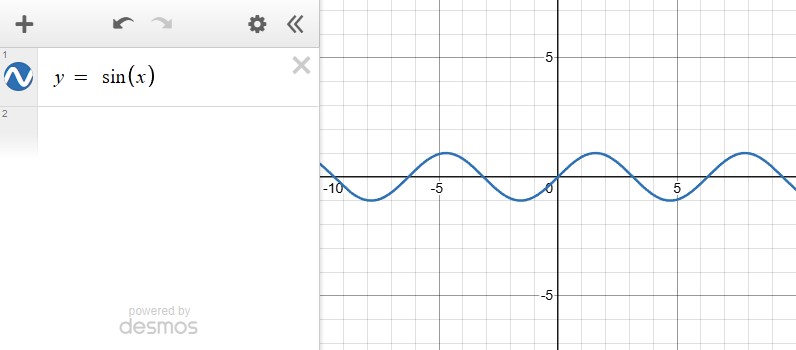
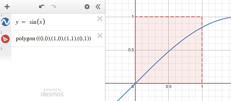
The previous shader successfully draws the shape of $\sin \left(x\right)$, but you might remember from Maths class that a sine is supposed to look like a wave. The shader is hiding most of the function!

This happens because the UV coordinates range between [0.0, 1.0]. Naturally, the shader will then draw the sine of values from that interval, revealing just a tiny slice of the function.

To get a better overview of a function you can make use of a graph plotting aplication to draw and analyze it. There are many such tools, but a commonly used one is the Desmos Graphing Calculator. You can use it in your browser to view any of the functions shown in this article.

Let's take a look at $\sin \left(x\right)$ in Desmos to reveal its wave-like shape:

Right now it's zoomed out, but as you get closer to the [0.0, 1.0] interval, the function starts to resemble the shape seen in the shader.

This looks very close to our shader. The only thing left to do is to flip the shader vertical axis, so that it goes up, just like the one in Desmos. You can do this by subtracting UV.y from 1.0:

void fragment() {
  vec2 uv = vec2(UV.x, 1.0 - UV.y);

  if (uv.y > sin(uv.x)) {
    discard;
  }

  COLOR = vec4(0.1, 0.3, 0.55, 1.0);
}

Why does subtracting y from 1.0 invert the axis?

To understand this it's best to see some examples in which we replace $y$ with $1.0-y$.

Take $0.2$. For this value, $1.0-0.2=0.8$. On the other hand, for $0.8$ you get $1.0-0.8=0.2$.

Apply this for all values between [0.0, 1.0] and you flip the whole axis.

Making a water shader

Now that everything is set up, let's use our blue shader to create a water effect. The sine function is already doing most of the work by providing a wave-like shape. It just needs to be scaled and translated so that the waves fit between 0.0 and 1.0.

You can change the shape of a function by multiplying or adding values to its parameters. Let's do that by replacing $y=\sin \left(x\right)$ with:

void fragment() {
  vec2 uv = vec2(UV.x, 1. - UV.y);

  if ((uv.y - 0.7) / 0.05 > sin(uv.x/0.05)) {
    discard;
  }

  COLOR = vec4(0.1, 0.3, 0.55, 1.0);
}

Wait, how did you come up with these values?

Instead of randomly guessing values until the wave looks right, it's better to find what causes a function to move and scale. This lets you adjust a function almost like you would position a Node inside a Godot scene.

The following section might look intimidating, but you don't need to memorize these formulas. You can always come back to it whenever you need a refresher.

1. Translation

Subtract a value $h$ from $x$ to move the function horizontally, and a value $v$ from $y$ to move it vertically:

$$y-v=f\left(x-h\right)$$

2. Scaling

Divide $x$ by a horizontal scale factor $h_s$ and $y$ by a vertical factor $v_s$ to scale a function:

$$\frac{y}{v_s}=f\left(\frac{x}{h_s}\right)$$

3. Combining Both

By combining translation and scaling, you get a function that can be moved and resized in any direction:

$$\frac{y-v}{v_s}=f\left(\frac{x-h}{h_s}\right)$$

This form is useful for comparisons, but sometimes you'll need to store the final result of the transformations inside of a variable. Apply the inverse operations to the terms on the left side to move them to the right side:

$$y=f\left(\frac{x-h}{h_s}\right)\cdot v_s+v$$

If you generalize the sine used in the shader you get a customizable wave. Play around with the sliders until you get a wave shape you like.

H

0

V

0.7

H S

0.05

V S

0.05

shader_type canvas_item;

uniform float h : hint_range(-3.14, 3.14) = 0.0;
uniform float v : hint_range(0, 1) = 0.7;

uniform float h_s : hint_range(0.01, 2) = 0.05;
uniform float v_s : hint_range(0.01, 2) = 0.05;

void fragment() {
  vec2 uv = vec2(UV.x, 1.0 - UV.y);

  if ((uv.y - v) / v_s > sin((uv.x - h) / h_s)) {
    discard;
  }

  COLOR = vec4(0.1, 0.3, 0.55, 1.0);
}

For the purposes of this guide, if you encounter a function with seemingly random values, just know it was created with the same technique: sliding and scaling until it reaches the right spot.

Learning how to control function behavior is essential for avoiding guesswork and getting the effects you want. You can read more about these techniques in the function control library article.

This already resembles a water surface. For some styles, a single repeating wave may be all you need. But real water contains waves of different sizes and speeds that overlap and interfere with one another. A single wave is too regular to capture that variation. You can create a more natural surface by combining multiple functions to make up a new wave.

There are three common methods used to combine functions:

• Addition: Add two functions together to create a new one that follows their combined path.
• Multiplication: Multiply two functions together to amplify or reduce one's effect by the other.
• Composition: Feed the output of one function into another for changing its input values.

All three aim to add variance and complexity to your shader effects.

Function Addition

This is the exact technique we'll use to make our simple wave look more convincing.

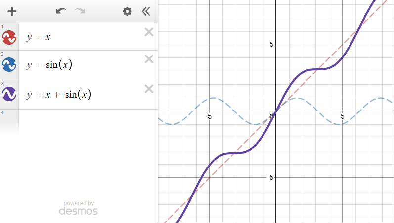
By adding two functions you make one function follow the path of the other.

Mathematically, at every single point $x$ along the horizontal axis, the vertical height is calculated from the first function. Then, the other function adds its height to that result.

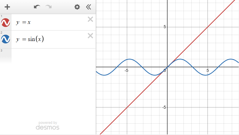
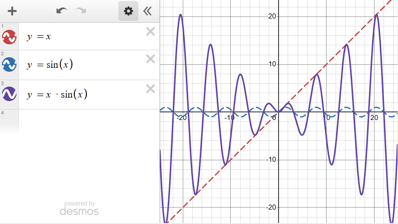
To see this clearly, let's start by plotting two completely different shapes in Desmos: a diagonal line $y=x$, and a sine wave $y=\sin \left(x\right)$.

Now, watch what happens when you add the two together:

The wave is no longer centered flatly around 0.0. Instead, it keeps its curvy shape, but uses the diagonal line as its new direction.

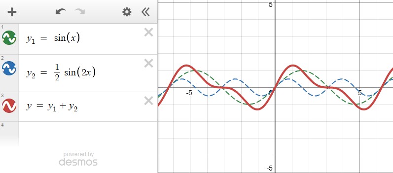
The same idea occurs when combining two waves together. You can use a large wave as the base shape of the water effect and a smaller wave that rides on top of it. This creates a ripple effect like the ones you see in real water.

The repeating pattern is still easy to spot, but it's much more visually interesting. It looks even better if you decrease the height of the waves and allow them to move horizontally at slightly different speeds:

You don't have to stop at two waves. You can make the pattern more natural by layering three, four or even more on top of each other. Just try to not overdo it. As the height of each new wave progressively decreases, its influence will become less and less noticeable.

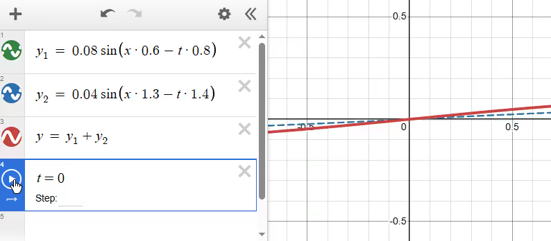
Let's add together three waves to the shader and animate them by subtracting the TIME built-in:

void fragment() {
  vec2 uv = vec2(UV.x, 1. - UV.y);
  
  float large_wave = 0.08 * sin(uv.x * 0.6 - TIME * 0.8);
  float medium_wave = 0.04 * sin(uv.x * 1.3 - TIME * 1.4);
  float small_wave = 0.02 * sin(uv.x * 2.8 - TIME * 3.3);

  float combined_wave = large_wave + medium_wave + small_wave;

  // 0.7 sets the base height of the combined wave
  if (uv.y - 0.7 > combined_wave) {
    discard;
  }

  COLOR = vec4(0.1, 0.3, 0.55, 1.0);
}

What combination of waves make for convincing water?

The rule of thumb for making convincing water is: the larger the wave, the smaller its parameters should be.

In the previous example, the largest wave is the one that's multiplied by 0.08. It should have a smooth frequency and move slowly. That's why we picked 0.6 for its frequency and multiplied the TIME built-in by 0.8 to get the speed at which to animate it.

For the rest of the waves, it's fine to halve the height and roughly double the frequency and animation speed. It's usually a good idea to be less precise when picking the doubles so that the waves have a smaller chance of overlapping.

Remember: You don't have to always be physically accurate when it comes to this kind of effects. Experiment and pick the values that fit your game!

Why is 0.7 in the comparison and not in the wave calculation?

It's easier to write and control a single value instead of three values that will end up added together.

If you only compare uv.y with the combined wave, you have to add $\frac{0.7}{3}$ to each wave, so that when added together they result in the 0.7 height we wanted for the water.

Function Multiplication

By multiplying two functions, you make one function scale the other.

This means that one of the functions will act as a base, while the other takes the role of a controller, deciding how strong the effect of the base should be.

• If the controller is 1.0, the base function stays at its full strength
• If the controller is 0.5, the strength of the base function is halved
• If the controller is 0.0, the base function has no effect

Just as before, let's take a look at the $y=x$ and $y=\sin \left(x\right)$ functions. Multiplying them together leads to a sine wave with an endleslly increasing amplitude:

Making a wind blown flag

Let's use function multiplication to make a fluttering flag. Along the way, you'll learn how to:

• Make a 2D texture look like a fabric fluttering in the wind
• Selectively animate parts of the flag with function multiplication
• Give the flag shadows that follow its folds

Heads up! We'll be using multiple techniques here

The techniques have been individually explained in the Shader Function Control. Go have a look if you need a refresher!

First you need to give the flag a texture. You can get textures inside a shader through a process called Texture Sampling.

Godot provides a texture() built-in function which allows a pixel to get the color of a texture at the provided coordinates. By default, a shader uses the TEXTURE and UV built-ins to get a CanvasItem's texture as it is.

void fragment() {
  COLOR = texture(TEXTURE, UV);
}

To make it seem like the flag flutters, add a sine based on the current fragment's horizontal position. To animate it, offset the oscillation by the passed TIME.

void fragment() {
  vec2 uv = UV;

  uv.y = uv.y + sin(uv.x - TIME);

  COLOR = texture(TEXTURE, uv);
}

The oscillation is too strong and the flag looks like it has an infinite surface.

Let's address the oscillation issue first. You can transform the sine with the same technique used before to create the water waves. As a reminder, this is the general formula for translating and scaling a sine:

To make the oscillation weaker, the sine can be multiplied by 0.2. You can also increase its frequency by multiplying the uv.x term by 4.0. The previous sine term can be replaced with this formula that we obtained by playing around with the generic, controllable version of the sine:

Each texture has a repeat mode which tells Godot what to do with it when a shader samples outside its coordinates. The infinite surface is caused by the default 'disabled' repeat mode of the texture.

When a texture doesn't repeat, the shader fills sampled colors outside its region with whatever color it found at the closest texture edge. Since all edges of the flag texture are purple, empty spaces get filled with purple as well. Discard all fragments outside the [0.0, 1.0] region to reveal the flag shape.

void fragment() {
  vec2 uv = UV;

  uv.y = uv.y + sin(uv.x * 4.0 - TIME) * 0.2;

  if (uv.x > 1.0 || uv.y > 1.0 || uv.x < 0.0 || uv.y < 0.0) {
    discard;
  }

  COLOR = texture(TEXTURE, uv);
}

The illusion breaks because the flag oscillates outside the shader boundaries. You can scale the flag down by multiplying the sampling coordinates. To keep everything in view, you need to scale from the center of the texture.Before scaling move the UVs left by 0.5 on both axes.

void fragment() {
  vec2 uv = UV;

  uv -= 0.5;
  uv = uv * 1.5;
  uv += 0.5;

  uv.y = uv.y + sin(uv.x * 4.0 - TIME) * 0.2;
  // ...
}

Why does the UV move left by 0.5?

By default, scaling or rotating UV coordinates happens relative to the origin point (0.0, 0.0). In Godot, this point represents the top-left corner of the texture.

The reason (0.0, 0.0) doesn't move is because the output for uv * 1.5 is still (0.0, 0.0). To choose the center (0.5, 0.5) of the UV coordinates as a scale pivot, you update the UVs to make that point land at (0.0, 0.0).

You can do that by subtracting 0.5 from both axes: uv -= 0.5. The UVs now range between [-0.5, 0.5], but their center is at (0.0, 0.0).

You can now scale by 1.5 to make the sampled result look smaller. Then, to sample correctly, you need to move the coordinates from [-0.5, 0.5] back to [0.0, 1.0]. You do that by adding back 0.5: uv += 0.5.

Now it's finally time to use function multiplication. Let's look again at $y=x\cdot \sin \left(x\right)$:

The oscillation strength keeps increasing, which fits nicely for a fluttering flag. But notice an important detail about the origin of the graph: when $x$ is $0.0$, the result is also $0.0$. This means there is no wave movement at all.

If you replace the sine from the shader with the sine multiplied by the horizontal coordinate, you keep the flag from moving where uv.x is equal to 0.0:

void fragment() {
  // ...
  uv.y = uv.y + sin(uv.x * 4.0 - TIME) * 0.2 * uv.x;
  // ...
}

The flag would look more believable with a shadow. To do that you need to multiply its color with a value that's smaller than 1.0. The only question is: Where to place the shadow?

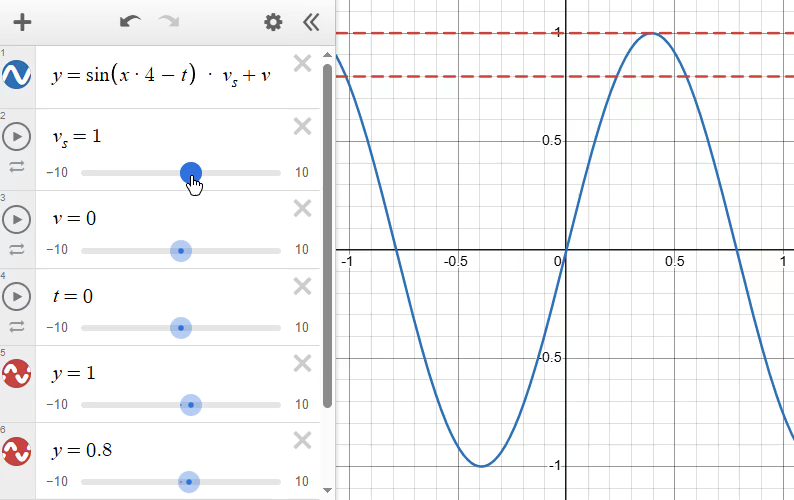
As the wind blows, it creates folds. These folds alternate between facing the light and facing away from it at the same rate the flag oscillates. Therefore, the shadow generates from the same wave that generated the oscillation: $\sin \left({\mathrm{uv}}_x\cdot 4.0-\mathrm{TIME}\right)$. This wave will be multiplied with the final color of the flag.

Let's make it so that the darkest shadow is 80% of the original color's brightness. For that, the wave needs to oscillate between [0.8, 1.0]. You already know how to do that! You just need to slide and scale the function vertically and you'll get:

You can add a uniform for the number of folds the flag will have and another for the wind speed. This transforms the wave from sin(uv.x * 4.0 - TIME) into sin(uv.x * folds - TIME * wind_speed).

Folds

6

Wind Speed

2

uniform float folds : hint_range(0.0, 20.0) = 6.0;
uniform float wind_speed : hint_range(1.0, 10.0) = 2.0;

void fragment() {
  vec2 uv = UV;

  uv -= 0.5;
  uv = uv * 1.5;
  uv += 0.5;

  uv.y = uv.y + sin(uv.x * folds - TIME * wind_speed) * 0.2 * uv.x;

  if (uv.x > 1.0 || uv.y > 1.0 || uv.x < 0.0 || uv.y < 0.0) {
    discard;
  }

  vec4 flag_color = texture(TEXTURE, uv);
  float shadow = sin(uv.x * folds - TIME * wind_speed) * 0.1 + 0.9;
  COLOR.rgb = flag_color.rgb * shadow;
  COLOR.a = 1.0;
}

Uniforms

Uniforms expose shader properties to the Godot Inspector. Define them in the global scope, outside any function:

uniform vec2 direction = vec2(0.0, 0.0);

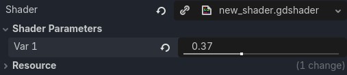
You can customize how they appear in the inspector by making use of uniform hints. A hint_range on a float produces a slider:

uniform float var1 : hint_range(0.0, 1.0) = 0.0;

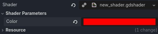
source_color on a vec4 produces a color picker:

uniform vec4 color : source_color = vec4(1.0, 0.0, 0.0, 1.0);

It's almost there! There's one thing left. Did you try increasing the number of folds? If you didn't, test it out and see if you notice the issue.

As you increase the number of folds, the flag seems to get larger and larger towards its right edge. This is because we chose a function that endlessly increases its oscillations: $y=x$. It looked good when the frequency was low, but, as we increase it, it starts falling apart.

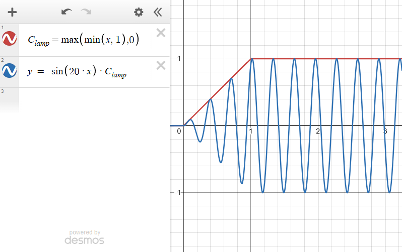
You can decide a point at which the sine should stop increasing by using the y = clamp(x, min, max) function, which limits $x$ (or any other function) between min and max.

Why is the function in Desmos different?

Desmos doesn't have a clamp function. However, it can easily be defined with min and max.

Since $x$ should be between 0.0 and 1.0, if $x$ is the minumum between itself and 1.0 and the maximum between itself and 0.0, then $x$ will only increase in the [0.0, 1.0] interval and clamp at the edges when it gets outside.

After you find the function, the change is simple: just replace uv.x with a clamp between 0.0 and a value at which the waves should peak, something like 0.5.

Folds

6

Wind Speed

2

uniform float folds : hint_range(0.0, 20.0) = 6.0;
uniform float wind_speed : hint_range(1.0, 10.0) = 2.0;

void fragment() {
  // ...
  uv.y = uv.y + 
    sin(uv.x * folds - TIME * wind_speed) * 0.2 * 
    clamp(uv.x, 0.0, 0.5);
  // ...
}

With the flag pinned, scaled, shaded and clamped, the effect is finally complete!

Through multiplication you learned to amplify or mute the effects of a function. This gives you better control over the shape and animations of your effects, even allowing you to selectively disable them.

But what if you wanted, not to change the strength of an effect, but the rate at which it varies? What if you wanted to make a wave start fast and then have it gradually slow down? For that you need to know function composition.

Function Composition

By composing two functions you use one to change the rate at which the other changes.

To compose two functions $\mathrm{y1}=f\left(x\right)$ and $\mathrm{y2}=g\left(x\right)$, you take the output of one and use it as the input of the other. Mathematically, you write this:

As opposed to the previous operations, this one doesn't give the same result when doing it in reverse. In math we say that the operation is not commutative. But this is a good thing, because you get a new effect when you write:

You actually use function composition every time you write a shader. When you write $y=\sin \left(x\right)$ you are secretly composing the linear function $y=x$ with the sine. This means that a function maintains its original form when composed with another one that grows steadily.

But what happens when you compose with a function that grows slower or faster than a linear one?

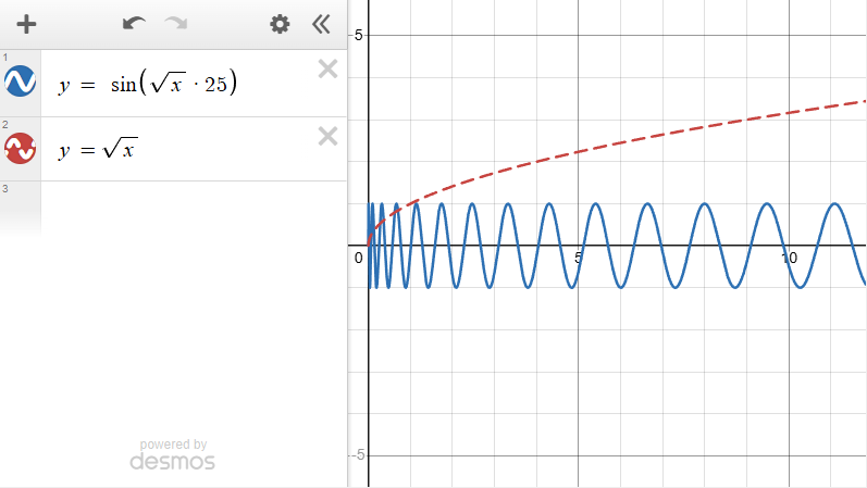
Let's see, for example, $y=\sqrt{x}$. It gets slower and slower the further $x$ is from $0.0$. When you compose it with a sine you get:

Because the square root curves flatter and flatter as $x$ increases, the wave's speed "decelerates". This makes the oscillations gradually decrease in frequency.

Why is the square root multiplied by 25?

The square root grows slowly. Multiplying by $25$ makes the effect seem more drastic and thus, easier to visualize.

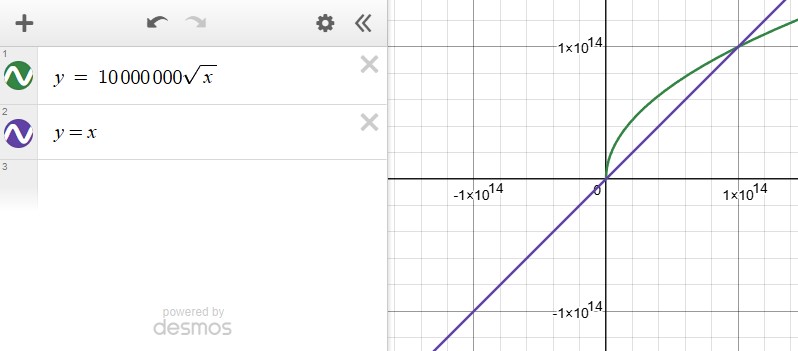
Multiplying or adding a constant value to a function doesn't change the rate at which it grows. For example, you could multiply $y=\sqrt{x}$ by ten million and it would still grow slower, and eventually be surpassed by $y=x$.

What about the opposite? What happens when you use a function like $y=x^2$ that grows faster than $y=x$? Compose it with the sine and you get:

It's as you'd expect: the wave starts slowly and accelerates the further right it goes.

But how can I combine functions I don't know of?

You do not need a degree in mathematics or a perfect memory of every function to be a great shader artist.

It's perfectly fine to learn as necessity arises. Once you know whether your effect needs to speed up, slow down, or oscillate, finding the right mathematical function is just a matter of looking for that specific behavior on a graph.

Making ripples with composition

The previous examples are especially useful for ripple-like effects. You can make a ripple by taking the distance from the center and plugging it into an animating sine function:

shader_type canvas_item;

void fragment() {
  float d = distance(UV, vec2(0.5));
  float rings = sin(d * 50.0 - TIME * 4.0);

  vec4 light_color = vec4(0.25, 0.40, 0.7, 1.0);
  vec4 dark_color = vec4(0.1, 0.3, 0.55, 1.0);

  COLOR = mix(light_color, dark_color, rings);
}

The distance() built-in

Godot provides a distance() built-in function that returns the distance between two points.

For example, distance(vec2(0.0, 0.0), vec2(0.5, 0.5)) returns the distance between the top-left corner and the center of the shader.

Inside the example shader we get the distance from the center and plug that into the sine. As the distance increases, the sine oscillates up and down:

float d = distance(UV, vec2(0.5));
float rings = sin(d * 50.0 - TIME * 4.0);

The mix() built-in

A mix() acts like a gradient between two values. Those values can be anything from floats to colors.

In the previous ripple effect the mix function is used to choose between two colors. Its third parameter tells the shader how much of each color to pick:

• When rings is 0.0 or less, mix returns the light_color
• When rings is 1.0 or more, mix returns the dark_color
• When rings is between 0.0 and 1.0, mix returns a blend of the colors. For example, if rings is 0.2, the result is 80% light_color and 20% dark_color

The way you obtain this third parameter dictates how the gradient will look like. If you simply plug in UV.x, you get a linear gradient between two colors:

shader_type canvas_item;

void fragment() {
  float blending_function = UV.x;

  vec4 light_color = vec4(1.0, 0.0, 0.0, 1.0);
  vec4 dark_color = vec4(0.0, 0.0, 1.0, 1.0);

  COLOR = mix(light_color, dark_color, blending_function);
}

But you can plug in any function to get different blends between these colors. For example, you can use $y=\sin \left(4\cdot \pi \cdot x\right)\cdot 0.5+0.5$ to get a repeating pattern of the two colors.

shader_type canvas_item;

void fragment() {
  float blending_function = sin(4.0 * PI * UV.x) * 0.5 + 0.5;

  vec4 light_color = vec4(1.0, 0.0, 0.0, 1.0);
  vec4 dark_color = vec4(0.0, 0.0, 1.0, 1.0);

  COLOR = mix(light_color, dark_color, blending_function);
}

While the ripples look neat, the spacing feels artificial. Real-world water ripples expand and disperse as they travel outwards.

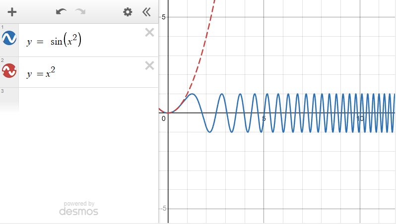
You can recreate this organic behavior by using function composition! Instead of feeding the linear distance $d$ into the sine wave, you can use the distance squared $d\cdot d$ instead.

shader_type canvas_item;

void fragment() {
  ...
  float rings = sin(d * d * 50.0 - TIME * 4.0);
  ...
}

You can also do the opposite! Replace the $d^2$ formula in the sine with $\sqrt{d}$. The wave squeezes the rings tighter as they get closer to the center, making it look like you're going through an endless tunnel.

shader_type canvas_item;

void fragment() {
  ...
  float rings = sin(sqrt(d) * 50.0 - TIME * 4.0);
  ...
}

Creating Retro, Pixelated Rings

You don't have to always go for realistic effects. The style of your game might require you to simplify shapes instead.

So far, all our examples relied on smooth, continuous functions. But these techniques apply to discontinuous functions as well. Let's take the initial ripple shader and make it look more like it came out of an arcade game:

shader_type canvas_item;

void fragment() {
  float d = distance(UV, vec2(0.5));
  float rings = sin(d * 50.0 - TIME * 4.0);

  vec4 light_color = vec4(0.25, 0.40, 0.7, 1.0);
  vec4 dark_color = vec4(0.1, 0.3, 0.55, 1.0);

  COLOR = mix(light_color, dark_color, rings);
}

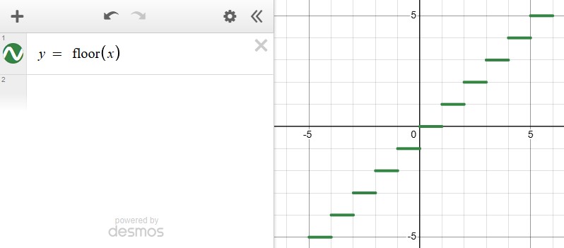
To achieve this we'll use the y = floor(x) function which returns the integer part of a floating point number. If you take a look at it in Desmos, it creates a staircase pattern:

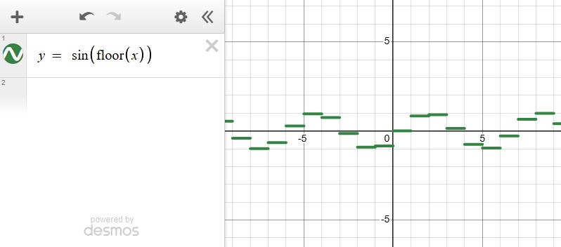
When you apply composition between y = sin(x) and y = floor(x), the resulting function looks like a staircase, but this time, it follows the sine wave. This happens because the sine no longer takes as inputs continuous values. Instead, the flat regions starting from 0.0 are the result of $\sin \left(1\right)$, $\sin \left(2\right)$, $\sin \left(3\right)$ and so on.

Let's see this effect in practice by replacing the rings generated with the sin(d * 50.0 - TIME * 4.0) function with the new floor composed function: sin(floor(d) - TIME * 4.0)

shader_type canvas_item;

void fragment() {
  ...
  float rings = sin(floor(d) - TIME * 4.0);
  ...
}

The effect just changes between the two shades of blue. This happens because of the distance used in calculating the floor.

Remember: the UV coordinates range between [0.0, 1.0]. The distance between any point in this range and the center will always be smaller than 1.0, making the floor always return 0.0. Because of that, the rings variable will be equal to sin(0 - TIME * 4.0). The TIME built-in shifts the sine, which changes the color, but the floor() function has no effect.

To make the effect work you need a floor function that returns at least two values. Let's multiply the distance by 2.0! This way, some distances will surpass 1.0 giving the floor() an additional value to return.

shader_type canvas_item;

void fragment() {
  ...
  float rings = sin(floor(d * 2.0) - TIME * 4.0);
  ...
}

This looks promising! With the floored distance returning either 0.0 or 1.0 the shader creates two bands. Let's make more of these bands by cranking the numbers up. Multiply the distance by 10.0 to get a low resolution pulsing wave:

shader_type canvas_item;

void fragment() {
  ...
  float rings = sin(floor(d * 10.0) - TIME * 4.0);
  ...
}

By placing a discontinuous function inside the inputs of another, you flattened regions of the base function and created a stylized effect.